Model compression reduces the size of a neural network (NN) without compromising accuracy. This size reduction is important because bigger NNs are difficult to deploy on resource-constrained devices. In this article, we will explore the benefits and drawbacks of 4 popular model compression techniques.
A brief history of model compression
In recent years, machine learning and deep learning have shown remarkable improvements in computer vision.
Let’s look at the evolution of deep neural networks in the last decade.
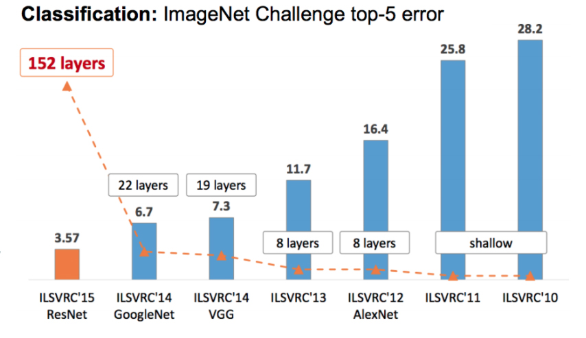
The chart above shows the top-5 error rate and number of layers of the winning models for the ImageNet challenge from 2010 to 2015.
In 2012, AlexNet won the ImageNet challenge with a very large margin improvement.
That was the turning point in computer vision history because it showed that deep neural networks (DNNs) could perform tasks that were considered very difficult for computers, not to mention that DNNs could do this with an unprecedented level of accuracy.
Each year, the accuracy of the winning models continued to increase, and so did their size.
The need for model compression
Many real-world applications demand real-time, on-device processing capabilities. For example, the AI on your home security camera must be able to process and notify you if there is someone unknown attempting to enter your house.
The main challenge with using state-of-the-art AI today is that the edge devices are resource-constrained. As a result, they have limited memory and limited processing capabilities.
The deep learning models that perform well are big in size. However, the bigger the model, the more storage space it needs, making it difficult to deploy on resource-constrained devices. Moreover, a bigger model means a higher inference time and more energy consumption during inference. While these models have achieved great results in the lab, they aren’t usable in many real-world applications.
That leaves us with one option: reducing the size of the model with AI compression.
Making a smaller model that can run under the constraints of edge devices is a key challenge. It’s also important to do this without compromising accuracy.
It is just not enough to have a small model that can run on resource-constrained devices. It should perform well, both in terms of accuracy and inference speed.
That’s where model compression or AI compression techniques come in.
4 Popular AI Compression Techniques
As the name suggests, model compression helps reduce the size of the neural network without compromising too much on accuracy.
The resulting models are both memory and energy efficient.
Many model compression techniques can be used to reduce the model size. This article will focus on four popular compression techniques:
- Pruning
- Quantization
- Knowledge distillation
- Low-rank factorization
1. The pruning technique
Pruning is a powerful technique to reduce the number of deep neural networks parameters. In DNNs, many parameters are redundant because they do not contribute much during training. So, after training, such parameters can be removed from the network with little effect on accuracy.
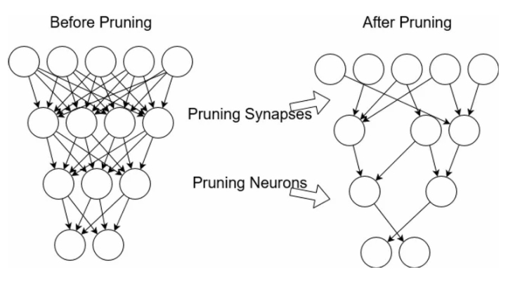
Pruning results in compressed models that run faster. It reduces the computational cost involved in network training and reduces the overall model size. Importantly, it also saves computation time and energy.
A model can be pruned during or after the training. Various techniques exist for this pruning process; some of these are:
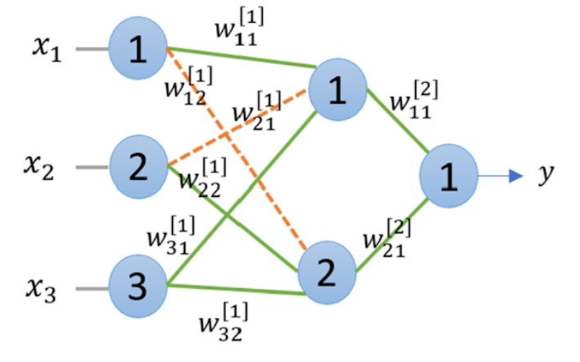
- Weight Pruning
Weight connections that are below some predefined thresholds are pruned (zeroed out).
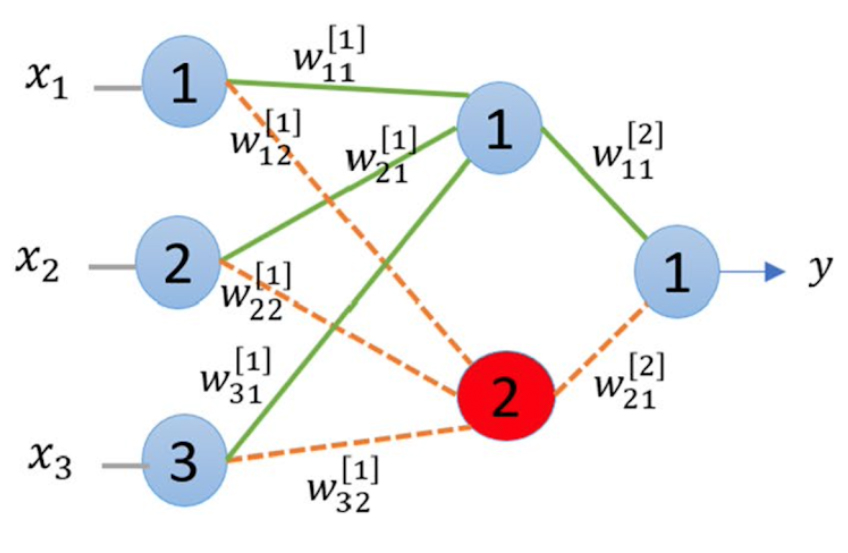
- Neuron Pruning
Instead of removing the weights one by one, which can be time-consuming, we prune the neurons.
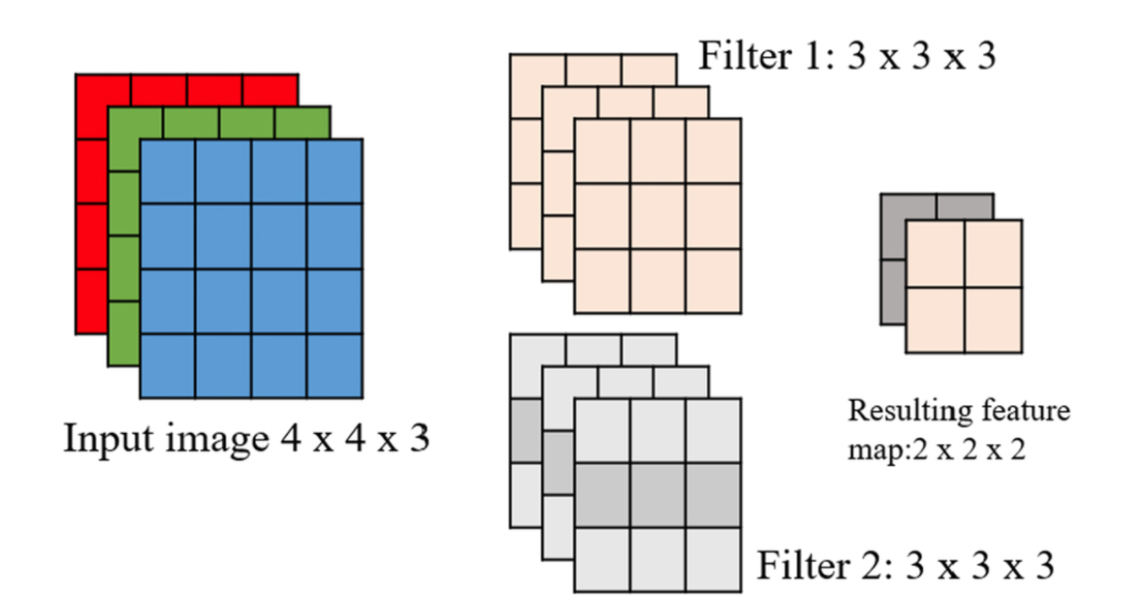
- Filter Pruning
Filters are ranked according to their importance, and the least important filters are removed from the network. The importance of the filters can be calculated by L1/L2 norm.
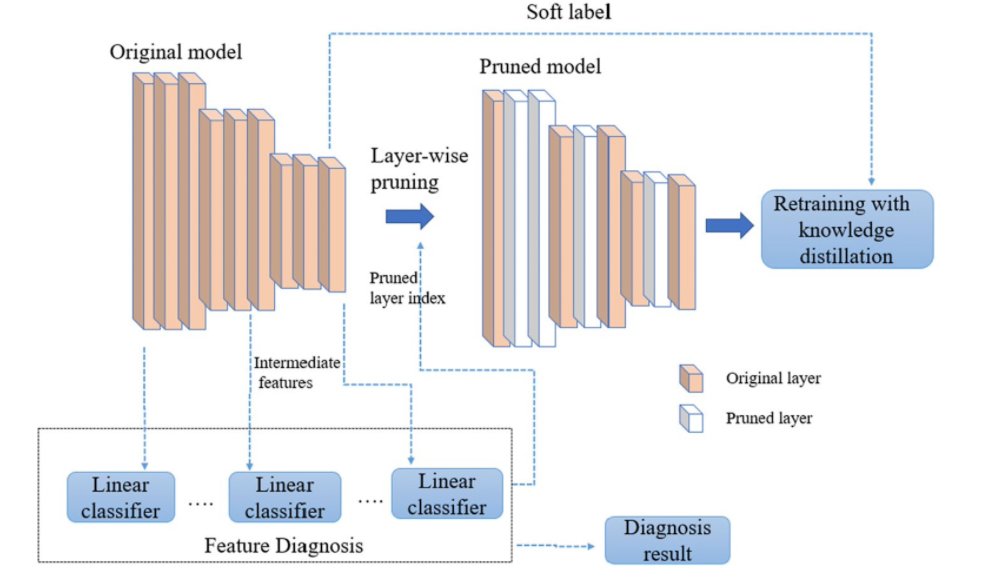
- Layer Pruning
Layers can also be pruned.
The graphs below show the size and speed vs accuracy trade-offs for different pruning methods and families of architectures.
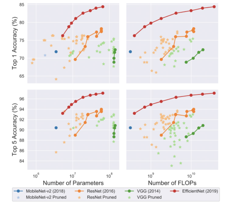
By looking at these graphs, we can observe that pruned models sometimes perform better than the original architecture, but they rarely outperform the better architecture.
To summarize, pruning can be applied during or after training. It can be applied to both convolutional and fully connected layers. Both the original and pruned model have the same architecture. Pruned models sometimes outperform the original architecture but rarely outperform a better architecture.
2. The quantization technique
In DNNs, weights are stored as 32-bit floating point numbers.

Quantization compresses the original network by reducing the number of bits required to represent each weight. For example, the weights can be quantized to 16-bit, 8-bit, 4-bit and even 1-bit. By reducing the number of bits used, the size of the DNN can be significantly reduced.
There are two forms of quantization. These are post-training quantization and quantization aware training.

Quantization can be applied both during and after training. It can be applied to both convolutional and fully connected layers. However, quantized weights make neural networks harder to converge and make back-propagation infeasible.
The table below shows the comparison of different DNN compression model compression techniques on the ImageNet dataset and standard pre-trained models.
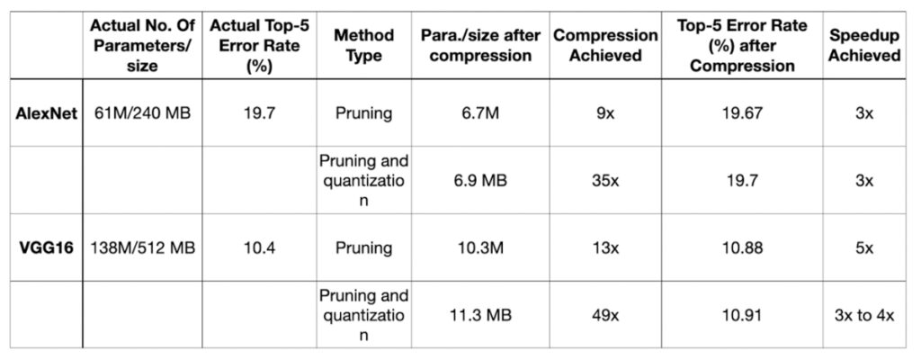
By using pruning on AlexNet, the resulting network was 9 times smaller and 3 times faster than the original network without any reduction in accuracy. When further quantization was applied, the resulting network was 35 times smaller and 3 times faster than the original network.
Similarly, VGG16 was reduced 13 times by applying pruning, which sped up the inference by 5 times without significantly reducing accuracy. When further quantization was applied, the size was reduced 49 times that of the original model.
3. The knowledge distillation technique
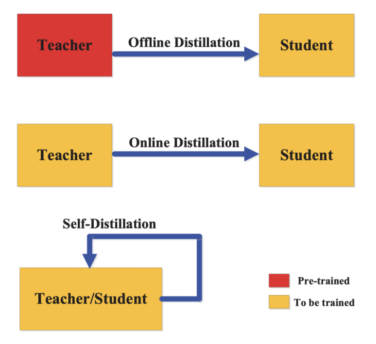
In knowledge distillation, a large, complex model is trained on a large dataset in knowledge distillation. When this model can generalize and perform well on unseen data, the knowledge is transferred to a smaller network. The larger model is known as the teacher model, and the smaller network is known as the student network.

In knowledge distillation, knowledge types, distillation strategies and the teacher-student architectures play a crucial role in the student learning.
Knowledge distillation is different from transfer learning, where we use the same model architecture and learned weights, and only replace some of the fully connected layers with new layers as per the requirements of the applications.
Currently, the knowledge distillation technique is limited to classification-based applications only.
It is challenging to train student networks from the teacher for tasks such as object detection and segmentation.
The activations, neurons or features of intermediate layers also can be used as the knowledge to guide the learning of the student model. Different forms of knowledge can be transferred. These are response-based knowledge, feature-based knowledge, and relation-based knowledge.
Different knowledge distillation strategies are:
- Offline distillation
- Online distillation
- Self-distillation
4. The low-rank factorization technique
Low-rank factorization identifies redundant parameters of deep neural networks by employing the matrix and tensor decomposition. When reducing the model size is necessary, a low-rank factorization technique helps by decomposing a large matrix into smaller matrices.
A weight matrix A with m x n dimension and having a rank r can be decomposed into smaller matrices.
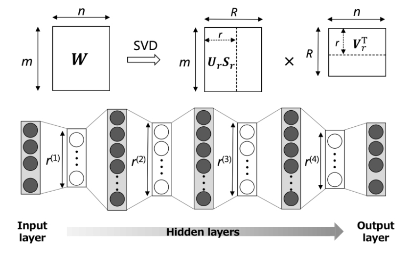
The low-rank factorization of the dense layer matrices mainly improves the storage requirements and makes the model storage-friendly, while the factorization of convolutional layers makes the inference process faster.
The accuracy and model performance depends on proper factorization and rank selection. Here, the main challenge is that the decomposition process results in harder implementations and is computationally intensive.
To summarize, low-rank factorization can be applied during or after training. Furthermore, it can be applied to both convolutional and fully connected layers. When applied during training, it can reduce training time. In addition, the factorization of the dense layer matrices reduces model size and improves speed up to 30-50% compared to the full-rank matrix representation.
Model compression and its challenges
The model compression and acceleration methods of DNNs have achieved significant momentum over the last couple of years. However, a major challenge that still exists with DNNs is finding the right balance between varying resource availability and system performance for resource-constrained devices.
Model compression techniques are complementary to each other. These techniques can be applied to pre-trained models as a post-processing step to reduce model size and increase inference speed. They can be applied during training time as well.
Pruning and Quantization have now been baked into machine learning frameworks such as Tensorflow and PyTorch.
There are many more compression approaches beyond the four common ones covered in this article, such as weight sharing-based model compression, structural matrix, transferred filters, and compact filters.

